risa 3d drawing elements are not correct

Solarian Programmer

My programming ramblings

OpenGL 101: Matrices - projection, view, model

Posted on May 22, 2013 by Paul

The lawmaking for this mail is on GitHub: https://github.com/sol-prog/OpenGL-101.

This is the fourth article from my OpenGL 101 series, if you need to refresh your memory you can find a listing with my previous articles at the cease of this post or, you can click on the OpenGL category from the right sidebar.

Until now we've used the default OpenGL view for cartoon our geometries and textures. While it is possible to draw any 2d geometry nosotros can think of using the default [-ane, +i] x [-ane, +1] space that OpenGL sets for us, information technology will quickly became cumbersome and inefficient. Consider the problem of cartoon four equilateral triangles, with unlike positions and orientations, like in the post-obit figure:

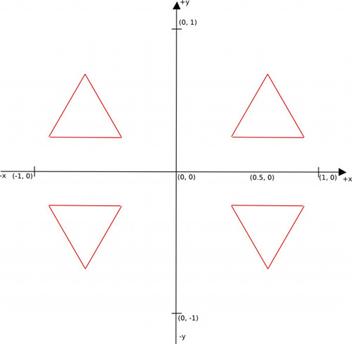
A possible solution is to store all four triangle coordinates in an assortment, like in our previous commodity. What if, instead of four we'd have twenty triangles spread on our screen ? In the after instance nosotros'll need to store lx vertices in our array. Now, imagine that you have a complex object made from a certain number of triangles, with his surface painted with one or more textures. Say that we want to replicate this object a few times on our screen at various positions and orientations. Clearly, we need a improve way to do this than to shop the object in all possible positions and orientations.

Fortunately for us, this is a solved trouble in computer graphics, just it involves a bit of matrix algebra. Instead of storing an object North times, we will store the object a single time and apply geometrical transformations similar translations, rotations and scaling to place the object where we need it.

In the adjacent figure we exemplify the concept of geometrical transformations using a foursquare:

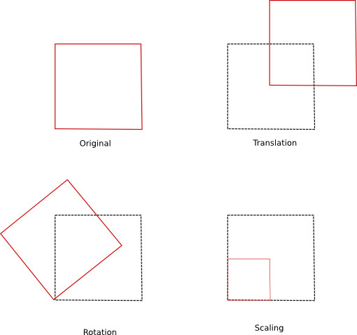
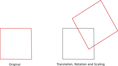
The above figure presents private transformations applied to a foursquare. These simple transformations can be combined, if we need to accomplish more circuitous transformations:

So, how do nosotros translate an object in our OpenGL lawmaking ? We offset, every bit usual, by transferring the object coordinates to an OpenGL buffer and we multiply the object coordinates with a translation matrix in the vertex shader program.

If you don't know what a matrix is or what matrix multiplication means, I've included a quick introduction in the next few paragraphs. You tin can use this as a quick refresher even if you've worked with matrix algebra concepts in the by. Please note that this is not an exhaustive presentation of matrix algebra, nosotros barely scratch the tip of the iceberg here. I've included at the end of this commodity a link to two good introductory books in matrix algebra for game design and computer graphics, if y'all want to acquire more nearly this subject.

Matrix algebra refresher

Mathematically, a matrix is a rectangular grid of numbers. We tin can identify a number, or an element, in a matrix by his respective row number and column.

\[\left[ {\begin{assortment}{*{xx}{c}} a&b&c&d \\ e&f&g&h \\ i&j&thousand&l \end{assortment}} \right]\]

For example h in the above matrix is on the 2nd row and fourth column.

We bespeak that a matrix M has chiliad rows and due north columns using the notation:

\[{M_{m,n}}\]

A matrix that has the number of rows equal to the number of columns is named foursquare.

We say that a square matrix is diagonal if all the elements are zero except for the ones from the main diagonal:

\[\left[ {\brainstorm{assortment}{*{20}{c}} a&0&0 \\ 0&b&0 \\ 0&0&c \end{array}} \right]\]

The identity matrix is a diagonal matrix with every diagonal element equal to 1, the identity matrix is ordinarily denoted as I:

\[I = \left[ {\begin{array}{*{xx}{c}} one&0&0 \\ 0&one&0 \\ 0&0&1 \terminate{array}} \right]\]

A matrix with north rows and 1 column is named a column vector:

\[\left[ {\begin{assortment}{*{xx}{c}} 1 \\ ii \\ 3 \end{assortment}} \right]\]

A matrix with i row and due north columns is named a row vector.

\[\left[ {\begin{array}{*{20}{c}} i&2&3&4 \stop{array}} \right]\]

Matrix transposition - if we have a matrix M with n rows and k columns, the transpose of \(M\), denoted \({M^T}\) is a matrix with thou rows and north columns, with the kickoff column of \({M^T}\) equal to the showtime row of \(M\) and and then on. Example:

\[M = \left[ {\begin{assortment}{*{20}{c}} a&b&c&d \\ due east&f&m&h \\ i&j&k&fifty \stop{array}} \right]\] \[{M^T} = \left[ {\begin{array}{*{xx}{c}} a&e&i \\ b&f&j \\ c&one thousand&k \\ d&h&l \end{array}} \correct]\]

As a side note, if nosotros transpose a column vector we obtain a row vector and vice-versa.

Matrix improver - two matrices of the same dimensions tin can exist summed, nosotros add them element by chemical element. Example:

\[\left[ {\begin{array}{*{twenty}{c}} 1&0 \\ 0&ane \finish{assortment}} \right] + \left[ {\begin{assortment}{*{20}{c}} 2&three \\ iv&v \cease{assortment}} \correct] = \left[ {\begin{assortment}{*{20}{c}} {ane + 2}&{0 + 3} \\ {0 + 4}&{ane + five} \stop{array}} \right] = \left[ {\begin{array}{*{twenty}{c}} iii&three \\ 4&6 \end{array}} \right]\]

For matrix subtraction we proceed in the same way, we subtract them element by chemical element. Example:

\[\left[ {\begin{array}{*{20}{c}} 1&0 \\ 0&one \stop{array}} \right] - \left[ {\begin{assortment}{*{20}{c}} 2&3 \\ 4&5 \stop{array}} \right] = \left[ {\brainstorm{array}{*{xx}{c}} {ane - 2}&{0 - 3} \\ {0 - 4}&{ane - five} \end{assortment}} \right] = \left[ {\begin{assortment}{*{20}{c}} { - i}&{ - 3} \\ { - 4}&{ - iv} \stop{array}} \right]\]

Matrix multiplication with a scalar (or matrix multiplication with a number) is the operation of multiplying every element of the matrix with a scalar. Example:

\[2 \cdot \left[ {\begin{assortment}{*{20}{c}} one&2&3 \\ 4&v&six \finish{array}} \right] = \left[ {\begin{array}{*{20}{c}} {two \cdot one}&{2 \cdot two}&{2 \cdot three} \\ {ii \cdot 4}&{ii \cdot five}&{2 \cdot 6} \end{array}} \right] = \left[ {\begin{array}{*{xx}{c}} 2&four&six \\ eight&{10}&{12} \end{array}} \right]\]

Matrix multiplication - if we take two matrices \({A_{m,n}}\) and \({B_{n,p}}\), the result of the multiplication is a new matrix \({C_{yard,p}}\). The starting time element of C can exist obtained by taking the first row of A and first cavalcade of B, multiplying them element by chemical element and summing the consequence. Second element of C, from the first line, can be obtained past multiplying the first line of A with the 2nd column of B and summing the result …

Example:

\[\left[ {\begin{array}{*{xx}{c}} i&2&3 \\ 2&four&0 \\ 5&{ - 1}&two \end{array}} \correct] \cdot \left[ {\begin{array}{*{20}{c}} 1&2 \\ 4&five \\ ane&0 \end{array}} \right] = \left[ {\begin{array}{*{20}{c}} {1 \cdot 1 + 2 \cdot 4 + 3 \cdot 1}&{1 \cdot 2 + two \cdot 5 + iii \cdot 0} \\ {two \cdot i + 4 \cdot four + 0 \cdot ane}&{2 \cdot 2 + 4 \cdot 5 + 0 \cdot 0} \\ {5 \cdot 1 - 1 \cdot four + 2 \cdot 1}&{5 \cdot 2 + ( - 1) \cdot 5 + 2 \cdot 0} \stop{array}} \correct] = \left[ {\begin{array}{*{20}{c}} {12}&{12} \\ {eighteen}&{24} \\ 3&v \finish{assortment}} \right]\]

In order to exist able to multiply ii matrices, A and B, the number of columns of A must exist equal to the number of rows of B. The resulting matrix will accept as dimensions - the number of rows of A and the number of columns of B. This is also suggested by the notation:

\[{A_{m,n}} \cdot {B_{n,p}} = {C_{m,p}}\]

Important properties of matrix multiplication:

• Matrix multiplication is not commutative, or, more explicitly, in general:

\[A \cdot B \ne B \cdot A\]

• Matrix multiplication is associative:

\[A \cdot B \cdot C = \left( {A \cdot B} \right) \cdot C = A \cdot \left( {B \cdot C} \right)\]

• The transpose of the product of two matrices is the product, in inverse order, of each matrix transposed:

\[{\left( {A \cdot B} \right)^T} = {B^T} \cdot {A^T}\]

An interesting property of the identity matrix is that:

\[A \cdot I = I \cdot A = A\]

Since a vector is basically a matrix (with dimensions 1xn or nx1), multiplying a vector with a matrix, or a matrix with a vector, obeys the same rules as the matrix multiplication. Examples:

\[\left[ {\brainstorm{array}{*{xx}{c}} ane&2&iii \\ 2&4&0 \\ 5&{ - 1}&2 \end{array}} \right] \cdot \left[ {\begin{assortment}{*{xx}{c}} ane \\ four \\ ane \end{assortment}} \right] = \left[ {\begin{assortment}{*{xx}{c}} {1 \cdot one + 2 \cdot 4 + 3 \cdot one} \\ {2 \cdot 1 + iv \cdot 4 + 0 \cdot 1} \\ {v \cdot one + ( - 1) \cdot 4 + 2 \cdot 1} \cease{array}} \right] = \left[ {\brainstorm{array}{*{20}{c}} {12} \\ {eighteen} \\ 3 \finish{array}} \right]\] \[\left[ {\brainstorm{assortment}{*{20}{c}} ane&4&1 \end{array}} \correct] \cdot \left[ {\brainstorm{array}{*{20}{c}} i&2&iii \\ two&four&0 \\ five&{ - ane}&2 \terminate{array}} \right] = \left[ {\begin{array}{*{20}{c}} {14}&{17}&5 \end{array}} \right]\]

The model matrix

As suggested earlier, we can apply various geometrical transformations on an object using matrices. If nosotros need to rotate an object, we multiply his coordinates with a rotation matrix, same goes for translation and scaling. The order in which we employ these transformations to an object is essential. We will achieve different effects if we interpret and apply a rotation to an object than if we start by rotating the object and translating the result.

From a mathematical indicate of view applying ii, or more, transformations to an object can be washed by multiplying the object coordinates with elementary matrix transformations 1 past one. Alternatively, nosotros can use a single matrix, that contains all the in a higher place transformations, to multiply the object coordinates:

\[R \cdot T \cdot 5 = M \cdot 5\]

where:

\[Thou = R \cdot T\]

and 5 is a cavalcade vector that contains a vertex from our object. In guild to properly transform an object, the transformation must be practical to every vertex of the object.

In the higher up equations we've replaced the product of two transform matrices, R (rotation) and T (translation), with a single transform matrix, M, using the associativity property of the matrix multiplication.

The matrix Grand, that contains every translations, rotations or scaling, applied to an object is named the model matrix in OpenGL. Basically, instead of sending down the OpenGL pipeline two, or more than, geometrical transformation matrices we'll send a single matrix for efficiency. Remember that the vertex shader program is executed for every vertex ? It is more efficient to multiply the coordinates of every vertex with a single model matrix than to practice it with two or more matrices.

Without further ado, these are the geometrical transformation matrices for a 3D vertex:

• Translation:

\[T = \left[ {\begin{array}{*{xx}{c}} 1&0&0&{T_x} \\ 0&1&0&{T_y} \\ 0&0&ane&{T_z} \\ 0&0&0&ane \end{assortment}} \right]\]

The to a higher place array will translate a vector, 5, with \({T_x}\) in the x direction, \({T_y}\) in the y management, etc …

• Rotation:

\[{R_x} = \left[ {\begin{array}{*{xx}{c}} one&0&0&0 \\ 0&{\cos \left( \blastoff \right)}&{ - \sin \left( \alpha \right)}&0 \\ 0&{\sin \left( \alpha \correct)}&{\cos \left( \alpha \right)}&0 \\ 0&0&0&1 \end{array}} \correct],\,\,{R_y} = \left[ {\begin{array}{*{20}{c}} {\cos \left( \alpha \correct)}&0&{\sin \left( \alpha \right)}&0 \\ 0&one&0&0 \\ { - \sin \left( \alpha \right)}&0&{\cos \left( \blastoff \right)}&0 \\ 0&0&0&1 \end{assortment}} \right],\,\,{R_z} = \left[ {\begin{array}{*{20}{c}} {\cos \left( \alpha \right)}&{ - \sin \left( \alpha \right)}&0&0 \\ {\sin \left( \alpha \right)}&{\cos \left( \blastoff \right)}&0&0 \\ 0&0&ane&0 \\ 0&0&0&1 \end{assortment}} \correct]\]

For rotation we have three matrices, respective to the Ox, Oy and Oz axes. For example, \({R_z}\) will rotate a vector v with \(\blastoff\) degrees around the Oz centrality counterclockwise.

• Scaling:

\[S = \left[ {\brainstorm{array}{*{twenty}{c}} {S_x}&0&0&0 \\ 0&{S_y}&0&0 \\ 0&0&{S_z}&0 \\ 0&0&0&1 \end{assortment}} \correct]\]

The above array will scale a vector, v, with \({S_x}\) in the 10 management, \({S_y}\) in the y direction, etc …

Delight note that the above matrices are 4x4 matrices and not 3x3 matrices! This is because the translation matrix can't be written as a 3x3 matrix and we use a mathematical fox to express the above transformations as matrix multiplications. An interesting consequence of working with 4x4 matrices instead of 3x3, is that nosotros can't multiply a 3D vertex, expressed as a 3x1 column vector, with the in a higher place matrices. Instead we'll utilise the and so called homogeneous coordinates, where a 3D vertex tin exist expressed every bit a 4x1 cavalcade vector. From our point of view, this only means that we'll write a 3D vertex every bit:

\[five = \left[ {\begin{assortment}{*{20}{c}} x \\ y \\ z \\ w \end{array}} \correct]\]

where w = ane.

If we want to transform a vertex from the homogeneous space to the 3D Cartesian infinite nosotros could utilise:

\[v = \left[ {\begin{assortment}{*{20}{c}} x/due west \\ y/w \\ z/w \terminate{assortment}} \right]\]

Permit's try, for e. g., to rotate a 2D vertex, x = 0.5 and y = 0.5, with \(\alpha = {90^\circ }\) around Oz:

\[\left[ {\brainstorm{array}{*{20}{c}} {\cos \left( {90 \cdot \frac{\pi }{180}} \right)}&{ - \sin \left( {90 \cdot \frac{\pi }{180}} \right)}&0&0 \\ {\sin \left( {90 \cdot \frac{\pi }{180}} \correct)}&{\cos \left( {ninety \cdot \frac{\pi }{180}} \correct)}&0&0 \\ 0&0&1&0 \\ 0&0&0&1 \end{array}} \right] \cdot \left[ {\brainstorm{array}{*{20}{c}} {0.5} \\ {0.5} \\ 0 \\ 1 \end{array}} \correct] = \left[ {\begin{array}{*{20}{c}} 0&{ - 1}&0&0 \\ 1&0&0&0 \\ 0&0&1&0 \\ 0&0&0&i \end{array}} \correct] \cdot \left[ {\begin{array}{*{20}{c}} {0.5} \\ {0.v} \\ 0 \\ 1 \end{array}} \right] = \left[ {\brainstorm{array}{*{20}{c}} { - 0.5} \\ {0.5} \\ 0 \\ 1 \stop{array}} \right]\]

The upshot of the above multiplication is the position of the rotated vertex, x = -0.5, y = 0.five. As a side note, I've transformed the bending from degrees to radians in the in a higher place matrix. As you lot probably know, you need to utilize radians for angles in lodge to use the trigonometrical functions in C or C++.

Say, that your intention was to interpret the vertex obtained after applying the above rotation with 0.1 on x, -0.two on y and 0.5 on z:

\[\left[ {\begin{assortment}{*{twenty}{c}} ane&0&0&{0.one} \\ 0&1&0&{ - 0.ii} \\ 0&0&1&{0.5} \\ 0&0&0&1 \end{array}} \right] \cdot \left[ {\begin{array}{*{xx}{c}} { - 0.5} \\ {0.5} \\ 0 \\ one \end{array}} \correct] = \left[ {\begin{array}{*{20}{c}} { - 0.four} \\ {0.3} \\ {0.5} \\ 1 \end{array}} \right]\]

Allow's write the above two transformations using the model matrix:

\[M = \left[ {\begin{array}{*{twenty}{c}} 1&0&0&{0.1} \\ 0&ane&0&{ - 0.2} \\ 0&0&1&{0.v} \\ 0&0&0&1 \end{assortment}} \correct] \cdot \left[ {\begin{array}{*{20}{c}} {\cos \left( {90 \cdot \frac{\pi }{180}} \right)}&{ - \sin \left( {ninety \cdot \frac{\pi }{180}} \right)}&0&0 \\ {\sin \left( {90 \cdot \frac{\pi }{180}} \right)}&{\cos \left( {xc \cdot \frac{\pi }{180}} \right)}&0&0 \\ 0&0&1&0 \\ 0&0&0&ane \end{array}} \right] = \\ = \left[ {\begin{array}{*{20}{c}} one&0&0&{0.1} \\ 0&1&0&{ - 0.2} \\ 0&0&ane&{0.v} \\ 0&0&0&1 \cease{array}} \right] \cdot \left[ {\begin{array}{*{20}{c}} 0&{ - 1}&0&0 \\ ane&0&0&0 \\ 0&0&1&0 \\ 0&0&0&i \cease{array}} \right] = \left[ {\begin{assortment}{*{twenty}{c}} 0&{ - one}&0&{0.1} \\ ane&0&0&{ - 0.2} \\ 0&0&1&{0.5} \\ 0&0&0&1 \end{array}} \right]\]

And now, we tin rotate and translate the original vertex with:

\[\left[ {\brainstorm{array}{*{20}{c}} 0&{ - 1}&0&{0.1} \\ 1&0&0&{ - 0.2} \\ 0&0&one&{0.5} \\ 0&0&0&1 \end{array}} \right] \cdot \left[ {\begin{array}{*{twenty}{c}} {0.5} \\ {0.5} \\ 0 \\ one \finish{assortment}} \right] = \left[ {\begin{array}{*{twenty}{c}} { - 0.4} \\ {0.3} \\ {0.v} \\ 1 \finish{array}} \correct]\]

The view matrix

By default, in OpenGL, the viewer is positioned on the z centrality, it is like using a camera to take a shot. Imagine that your photographic camera points to the origin of the Cartesian organization. The up direction is parallel to the Oy axis and in the positive sense of Oy.

The view matrix in OpenGL controls the way we expect at a scene. In this article nosotros are going to use a view matrix that simulates a moving photographic camera, usually named lookAt.

It is beyond the purpose of the present article to derive and present the way we create the view matrix, suffice to say that it is a 4x4 matrix, like the model matrix, and it is uniquely determined by three parameters:

• The eye, or the position of the viewer;

• The middle, or the betoken where we the photographic camera aims;

• The up, which defines the direction of the up for the viewer.

The defaults in OpenGL are: the eye at (0, 0, -1); the center at (0, 0, 0) and the up is given past the positive management of the Oy centrality (0, 1, 0).

Suppose that we have a generic C++ function that given the heart, the centre and the up will return a 4x4 view matrix for us.

The view matrix, V, multiplies the model matrix and, basically aligns the world (the objects from a scene) to the camera. For a generic vertex, v, this is the way nosotros apply the view and model transformations:

\[v' = V \cdot M \cdot v\]

The projection matrix

Past default, in OpenGL, an object volition appear to accept the same size no affair where the camera is positioned. This is against our twenty-four hour period to day experience, where an object closer to us (to the camera) looks larger than an object that is at a greater altitude. Picture the way a ball approaches you lot, the brawl volition announced bigger and bigger as it is closer to your eyes.

Another problem with the defaults from OpenGL is that in order to actually encounter (draw) something on the screen, the objects that we intend to draw must be inside the cube [-one, +ane] 10 [-i, +i] x [-1, +1]. Any part of our scene that is outside the unit cube will be clipped.

We tin well-nigh enlarge or shrink the clipping volume through the utilize of a project matrix, when our clipping volume has the shape of a parallelepiped, or a box, nosotros say that we use an orthographic projection. The orthographic projection will not modify the size of the objects no affair where the camera is positioned. This is a desirable feature for CAD programs or for 2D games.

The orthographic projection matrix:

\[P = \left[ {\brainstorm{array}{*{twenty}{c}} {\frac{2}{right - left}}&0&0&{ - \frac{correct + left}{right - left}} \\ 0&{\frac{2}{tiptop - bottom}}&0&{ - \frac{acme + lesser}{pinnacle - bottom}} \\ 0&0&{ - \frac{2}{far - almost}}&{ - \frac{far + about}{far - near}} \\ 0&0&0&1 \end{assortment}} \correct]\]

Where right, left, far, near, peak, bottom represents the positions of the clipping planes. Can yous approximate what is the orthographic projection matrix used by default in OpenGL. Hint, use the cube [-ane, +1] x [-1, +1] x [-1, +1] to define your right, left …

Another projection matrix, that can enhance the feeling of real world is the perspective projection matrix, in this example the book is a frustum and not a parallelepiped.

The perspective project matrix is:

\[P = \left[ {\begin{assortment}{*{twenty}{c}} {\frac{ii \cdot near}{right - left}}&0&{\frac{right + left}{right - left}}&0 \\ 0&{\frac{2 \cdot near}{acme - bottom}}&{\frac{acme + bottom}{tiptop - bottom}}&0 \\ 0&0&{ - \frac{far + near}{far - near}}&{ - \frac{2 \cdot far \cdot nearly}{far - almost}} \\ 0&0&{ - 1}&0 \end{array}} \right]\]

The perspective projection matrix is usually specified through iv parameters:

• viewing angle or field of view (usually abbreviated as FOV);

• aspect

• near and far

Where near and far represent the positions of the near and the far clipping planes.

\[\brainstorm{gathered} top = near \cdot \tan \left( {\frac{\pi }{180} \cdot FOV/2} \right) \\ bottom = - top \\ right = summit \cdot aspect \\ left = - right \\ \end{gathered}\]

The projection matrix, P, multiplies the production view matrix model matrix and, basically projects the earth coordinates to the unit cube. For a generic vertex, five, this is the style we apply the view and model transformations:

\[five' = P \cdot V \cdot M \cdot v\]

Putting the transformations at work

If you lot remember, in the first commodity of the OpenGL 101 serial, I've mentioned the GLM library. GLM is a small-scale mathematical library that implements the transformations presented in this commodity, matrix/vector operations and much more.

We'll start with a slightly modified version of ex_11 from our previous commodity. You volition find the complete source code for this article on Github.

Relieve the project as ex_14 and add the necessary GLM headers to the code:

                                                    1                                    #include                  <glm/glm.hpp>                                    2                                    #include                  <glm/gtc/matrix_transform.hpp>                                    iii                                    #include                  <glm/gtc/type_ptr.hpp>                                                

In the initialize role nosotros beginning by creating the model, view and projection matrices:

                                                    1                                    glm                  ::                  mat4                  Model                  ,                  View                  ,                  Project                  ;                              

After cosmos, the in a higher place matrices are equal to the identity matrix.

In order to transfer the in a higher place 3 matrices to the vertex shader we'll add at the end the initialization part:

                                                    one                                    // Transfer the transformation matrices to the shader program                  2                                    GLint                  model                  =                  glGetUniformLocation                  (                  shaderProgram                  ,                  "Model"                  );                  3                                    glUniformMatrix4fv                  (                  model                  ,                  1                  ,                  GL_FALSE                  ,                  glm                  ::                  value_ptr                  (                  Model                  ));                  4                                    5                                    GLint                  view                  =                  glGetUniformLocation                  (                  shaderProgram                  ,                  "View"                  );                  six                                    glUniformMatrix4fv                  (                  view                  ,                  1                  ,                  GL_FALSE                  ,                  glm                  ::                  value_ptr                  (                  View                  ));                  vii                                    8                                    GLint                  project                  =                  glGetUniformLocation                  (                  shaderProgram                  ,                  "Projection"                  );                  ix                                    glUniformMatrix4fv                  (                  project                  ,                  1                  ,                  GL_FALSE                  ,                  glm                  ::                  value_ptr                  (                  Projection                  ));                              

And the modified vertex shader programme:

                                                                        one                                    #version 150                                      ii                                                        3                                    in                  vec4                  position                  ;                                      iv                                    in                  vec2                  texture_coord                  ;                                      5                                    out                  vec2                  texture_coord_from_vshader                  ;                                      six                                                        seven                                    compatible                  mat4                  Model                  ;                                      eight                                    uniform                  mat4                  View                  ;                                      9                                    uniform                  mat4                  Project                  ;                  10                                    xi                                    void                  main                  ()                  {                  12                                    gl_Position                  =                  Projection                  *                  View                  *                  Model                  *                  position                  ;                  thirteen                                    texture_coord_from_vshader                  =                  texture_coord                  ;                  14                                    }                              

Line 12 from the vertex programme applies the transformation matrices to every vertex that enter the shader.

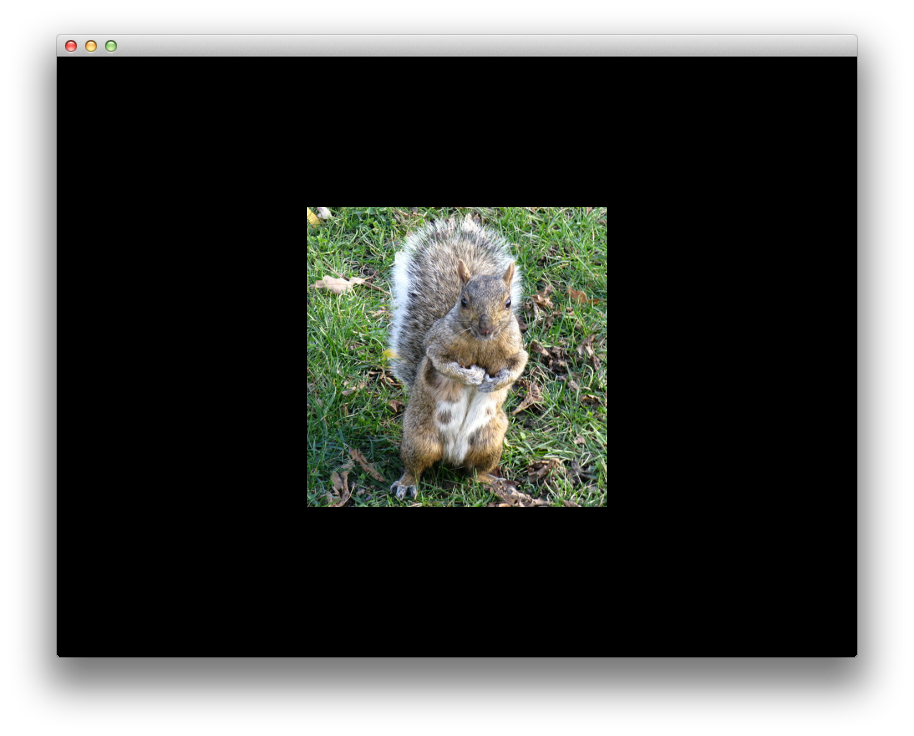
If y'all run the above code, this is what you should see:

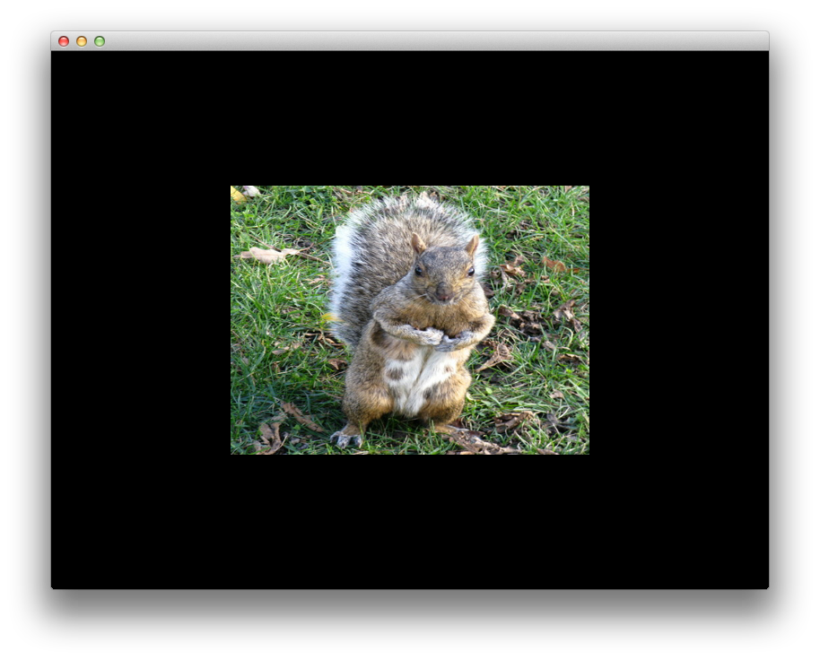
Obviously, the object is not altered past our unitary matrices multiplications. However, the square from the heart of the epitome looks more like a rectangle. This is because the attribute ratio of our window 800:600 will distort the length of whatever segment that is not parallel with the Oy axis. We tin correct this consequence in ii ways:

• Using a window with a 1:ane aspect ratio;

• Using the projection matrix to recoup the distortion of our window.

Let'south effort to employ the 2d solution, we get-go past imposing:

\[\frac{width}{height} = \frac{correct - left}{peak-lesser}\]

We fix the width, superlative, top, bottom and we have:

\[right - left = \frac{width \cdot (summit - bottom)}{height}\]

from where:

\[correct = \frac{width \cdot (tiptop - bottom)}{2 \cdot height}\]

and

\[left = -right\]

GLM allow united states to create a project matrix with glm::ortho(left, correct, lesser, meridian, near, far), in our particular case we tin use:

                                                    ane                                    glm                  ::                  mat4                  Model                  ,                  View                  ,                  Projection                  ;                  ii                                    3                                    // Fix the projection matrix                  four                                    Projection                  =                  glm                  ::                  ortho                  (                  -                  iv.0f                  /                  iii.0f                  ,                  4.0f                  /                  three.0f                  ,                  -                  1.0f                  ,                  i.0f                  ,                  -                  1.0f                  ,                  1.0f                  );                              

If you run the to a higher place code, you should see:

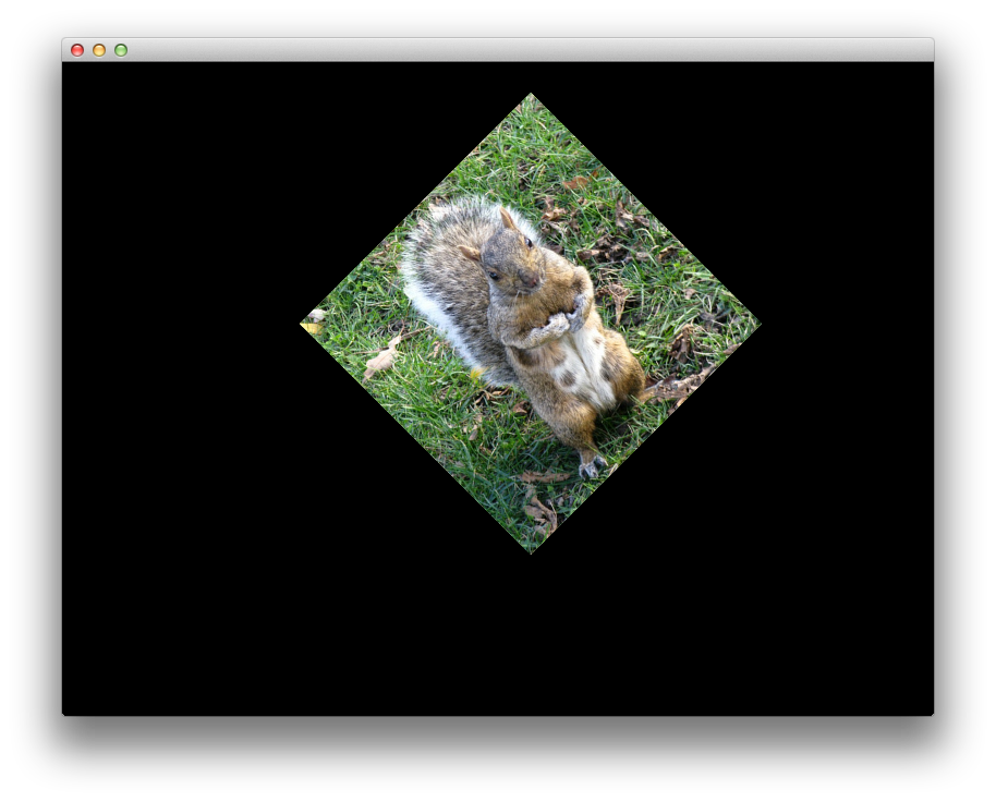
Let's apply a translation and a 45 degrees rotation to our object.

                                                                        1                                    glm                  ::                  mat4                  Model                  ,                  View                  ,                  Projection                  ;                                      2                                                        3                                    // Set the project matrix                                      4                                    Projection                  =                  glm                  ::                  ortho                  (                  -                  4.0f                  /                  three.0f                  ,                  4.0f                  /                  3.0f                  ,                  -                  1.0f                  ,                  1.0f                  ,                  -                  1.0f                  ,                  one.0f                  );                                      five                                                        half-dozen                                    // Translation                                      7                                    Model                  =                  glm                  ::                  translate                  (                  Model                  ,                  glm                  ::                  vec3                  (                  0.1f                  ,                  0.2f                  ,                  0.5f                  ));                                      8                                                        9                                    // Rotation around Oz with 45 degrees                  10                                    Model                  =                  glm                  ::                  rotate                  (                  Model                  ,                  45.0f                  ,                  glm                  ::                  vec3                  (                  0.0f                  ,                  0.0f                  ,                  1.0f                  ));                              

At line 7 glm::translate expects as parameters: the model matrix, and a vector with where y'all want the object to be translated \(T_x, T_y, T_z\), corresponding to the translation matrix presented earlier.

glm::rotate expects as parameters: the model matrix, the rotation angle in degrees and the rotation axis.

Please notation that GLM expects the angles in degrees, while the default in C++ is to apply the angles in radians.

If you run the above code, you should encounter:

In the adjacent article we are going to commencement drawing 3D bodies.

All posts from this serial:

• OpenGL 101: Windows, Bone X and Linux - Getting Started
• OpenGL 101: Drawing primitives - points, lines and triangles
• OpenGL 101: Textures
• OpenGL 101: Matrices - projection, view, model

If y'all are interested in learning more about Math for computer graphics and game programming, I would recommend reading Mathematics for 3D Game Programming and Computer Graphics by Eric Lengyel:

Another adept book most Math in computer graphics and game programming is 3D Math Primer for Graphics and Game Development past F. Dunn and I. Parberry:

A good book about modern OpenGL is OpenGL SuperBible by G. Sellers, S Wright and N. Haemel:

---

givenagdocany.blogspot.com

Source: https://solarianprogrammer.com/2013/05/22/opengl-101-matrices-projection-view-model/

Share this post